Curvature
Today will be all about curvature. Specifically, we will be looking at the Riemann curvature tensor and something called Ricci curvature.
Let’s begin with a heuristic approach before we dive into the formal definitions. What is curvature? You might have some sort of an idea about what it is for example it might not be too difficult for you to convince yourself that the following surface has some curvature.
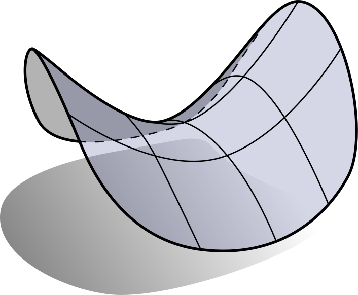
You might even know a method to quantify curvature from your background in vector analysis. Indeed the Frenet frame gives you a way to quantify curvature, but we are now in the realm of Riemannian Geometry and have moved on from the extrinsic geometry which is required for the Frenet frame.
So how can we come up with a method to capture this curviness of a manifold in an intrinsic way? Here is an idea, if $(M,g)$ is a Riemannian manifold, then we know that there exists a unique connection $\nabla$ which is compatible with $g$ i.e. the Levi-Civita connection. Given the connection, we have the ability to transport vectors since we can define the so-called parallel transport which we have discussed before. Maybe the transportation captures the curvature of the manifold somehow? Let’s investigate this.
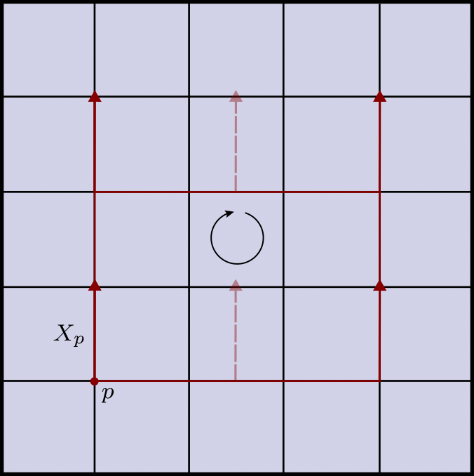
Consider first the manifold $\Bbb R^2$ with the usual Riemannian metric. Again heuristically speaking, we would expect this space to be flat even though we don’t yet know how to address this properly. Fix a point $p$ in $\Bbb R^2$, coordinates $(x^1,x^2)$ and consider a vector $X_p$ emanating from $p$. Observe now the following: transporting this vector first along the $x^2$-direction and then along the $x^1$-direction back to the point $p$ yields the same vector as the one we started with. The following illustration depicts this.
This innocent idea that you might even consider obvious turns out to be of utmost importance. Let’s now consider a manifold like $\Bbb S^2$ which you probably expect to have some sort of curvature. Fix again a point $p$ on the equator, and pick a vector $X_p$ emanating from $p$ and start transporting it around a closed spherical triangle. We see that the resulting vector is different than the vector we started with. Again the following illustration depicts this phenomenon.
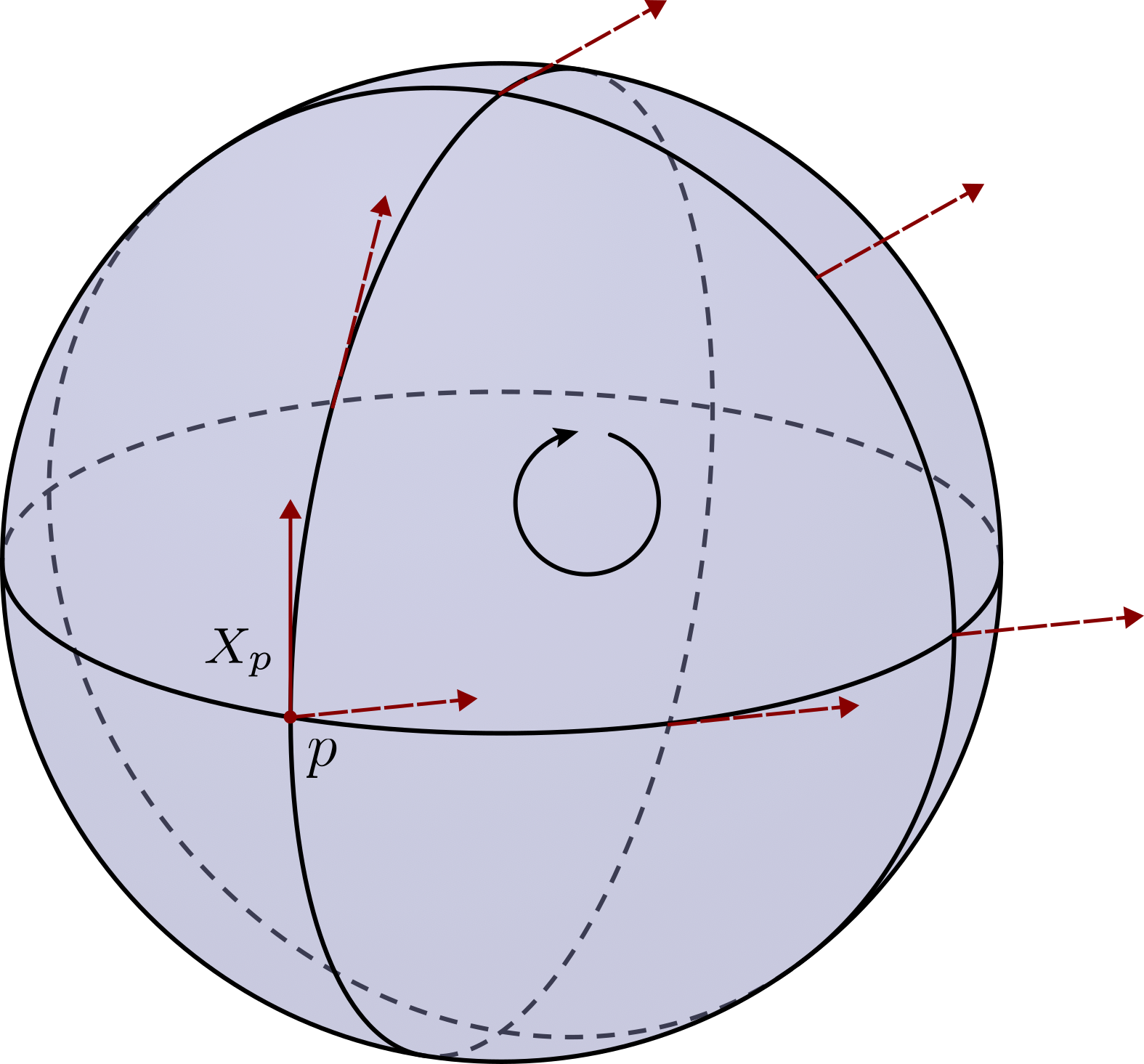
Aha! Seems like we are onto something. It’s exactly this curviness that $\Bbb S^2$ has and $\Bbb R^2$ doesn’t which is causing the transported vectors to be different. Motivated by this we can define curvature such that it measures in some sense how far away the connection is from being the standard connection on the Euclidean space. Said differently it should measure the deviation from local flatness1.
So how exactly should we go about defining curvature? Let’s look at the situation a bit more closely with the $2$-manifolds $\Bbb R^2$ and $\Bbb S^2$.
Beginning with $\Bbb R^2$ consider a point $p \in \Bbb R^2$ and a vector $X_p$ emanating from $p$.
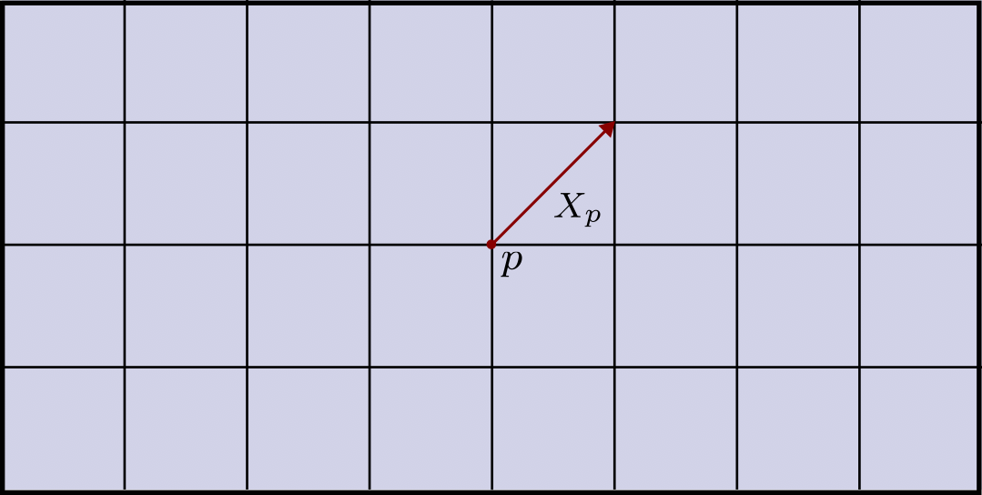
We can now try to create a parallel extension of $X_p$ in the following manner. Fixing a coordinate system $(x^1,x^2)$, first parallel transport $X_p$ along the $x^1$-axis and then parallel transport each of the resulting vectors along the coordinate lines parallel to the $x^2$-axis. We end up with a vector field $X$ that looks as follows.
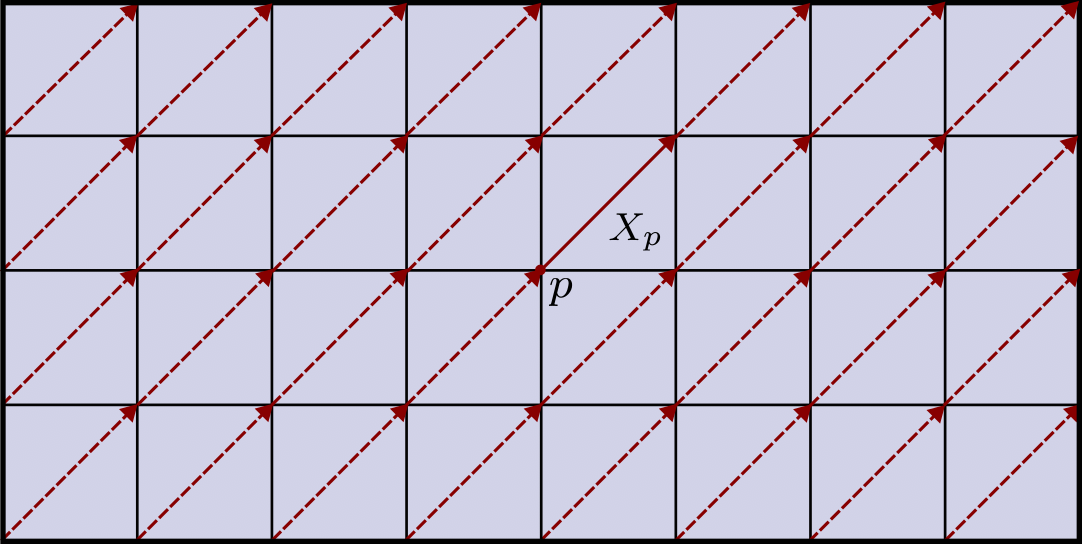
Now given our construction, $X$ is parallel along every $x^2$-coordinate line i.e. $\overline\nabla_{\partial_2} X = 0$ where $\overline\nabla$ is the standard Euclidean connection. When $x^2 = 0$ we have $\overline\nabla_{\partial_1} X = 0$. The question is now whether or not $X$ is parallel along every other $x^1$-coordinate line? Of course from our picture it’s clear, but we need to justify this. Notice that
\[\overline\nabla_{\partial_2}(\overline\nabla_{\partial_1} X) = 0 \implies \overline\nabla_{\partial_1} X = 0\]by the uniqueness of parallel transports. Here is where the flatness of $\Bbb R^2$ comes into play. $\Bbb R^2$ is special in the sense that
\[\begin{align*} \overline\nabla_{\partial_2}(\overline\nabla_{\partial_1} X) &= \overline\nabla_{\partial_2}\left((\partial_1 X^k)\partial_k\right) \\ &= (\partial_2\partial_1 X^k)\partial_k \\ &= (\partial_1\partial_2 X^k)\partial_k \\ &= \overline\nabla_{\partial_1}(\overline\nabla_{\partial_2} X) \end{align*}\]and as $\overline\nabla_{\partial_2} X = 0$ everywhere, we conclude that $\overline\nabla_{\partial_2}(\overline\nabla_{\partial_1} X) = 0$ i.e. $\overline\nabla_{\partial_1} X = 0$ everywhere. This essentially means that it doesn’t matter whether we parallel translate along $x^2$ first, and then along $x^1$ or vice versa.
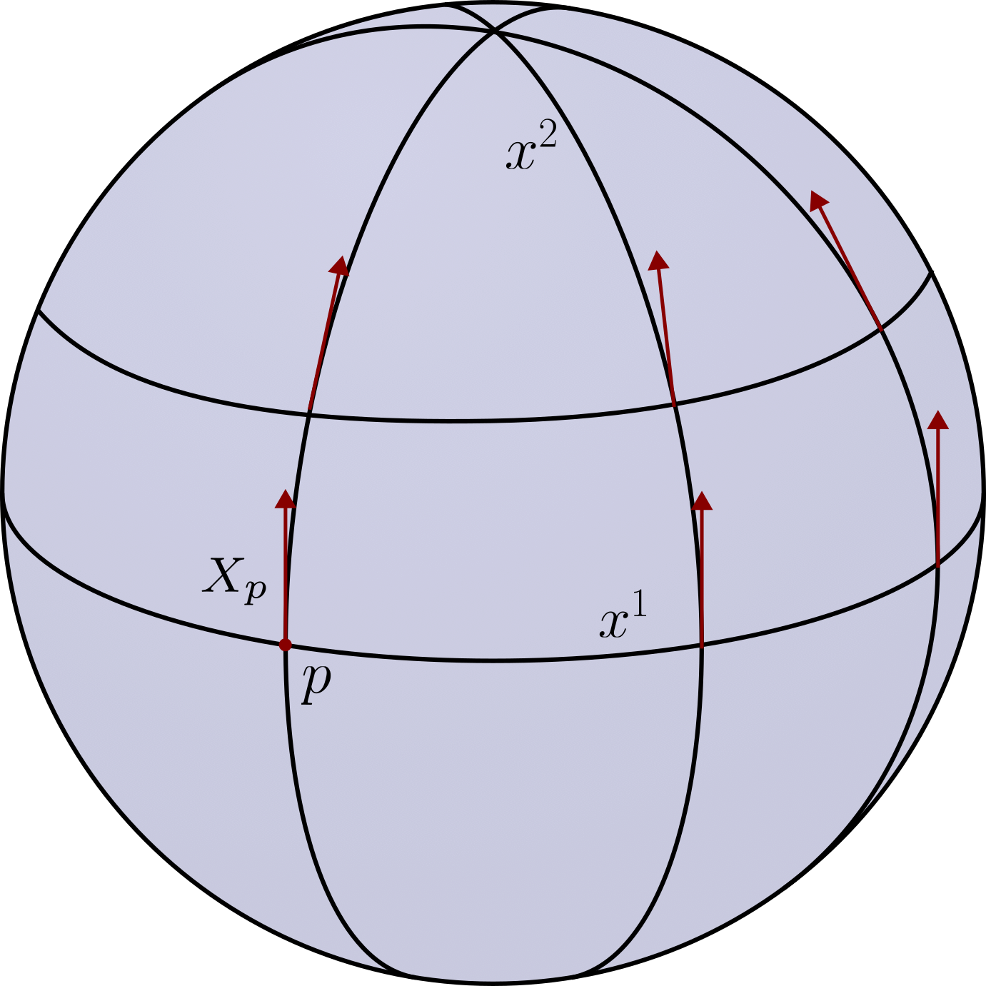
Again the situation changes drastically when we consider a curved space such as $\Bbb S^2$. Hopefully, you can convince yourself from the image below that the equation $\nabla_{\partial_2}(\nabla_{\partial_1} X) = \nabla_{\partial_1}(\nabla_{\partial_2} X)$ need not hold for the sphere.
More generally, on $\Bbb R^n$ for vector fields $X,Y,Z \in \Gamma(T\Bbb R^n)$ we have that:
\[\begin{align*} \overline\nabla_X \nabla_Y Z &= \overline\nabla_X(Y(Z^k)\partial_k) \\ &= XY(Z^k)\partial_k \end{align*}\]and likewise
\[\begin{align*} \overline\nabla_Y \nabla_X Z &= \overline\nabla_Y(X(Z^k)\partial_k) \\ &= YX(Z^k)\partial_k. \end{align*}\]Looking at the difference we see
\[\begin{align*} \overline\nabla_X \overline\nabla_Y Z - \overline\nabla_Y \overline\nabla_X Z &= XY(Z^k)\partial_k - YX(Z^k)\partial_k \\ &= (XY(Z^k) - YX(Z^k))\partial_k \\ &= \overline\nabla_{[X,Y]}Z. \end{align*}\]So in $\Bbb R^n$ the equality $\overline\nabla_X \overline\nabla_Y Z - \overline\nabla_Y \overline\nabla_X Z = \overline\nabla_{[X,Y]}Z$ holds for all vector fields $X,Y$ and $Z$ defined on an open subset of $\Bbb R^n$.
As we discussed above we want to define curvature such that measures the deviation from flatness. Well, now we have an expression that gives us exactly this. We say that a connection $\nabla$ on a Riemannian manifold satisfies the flatness criterion if
\[\nabla_X \nabla_Y Z - \nabla_Y \nabla_X Z = \nabla_{[X,Y]}Z\]holds for $X,Y,Z \in \Gamma(TM)$. Since the Levi-Civita connection is natural2, if $M$ is flat, then $\nabla$ satisfies the flatness criterion. All in all we have managed to come up with a necessary condition for a Riemannian manifold to be flat.
Let’s get on with the formalities then. Motivated by the above discussions we define the Riemann curvature endomorphism $R : \Gamma(TM) \times \Gamma(TM)\times \Gamma(TM) \to \Gamma(TM)$ by
\[R(X,Y)Z = \nabla_X \nabla_Y Z - \nabla_Y \nabla_X Z - \nabla_{[X,Y]}Z.\]As usual, when you meet an expression like this you should be asking yourself whether or not you are dealing with a tensor field.
As a $(1,3)$-tensor field, we can write $R$ in any local frame with one upper and three lower indices. In local coordinates $(x^i)$ we have:
\[R = R^l_{ijk} dx^i \otimes dx^j \otimes dx^k \otimes \partial_l.\]Occasionally its useful to lower the upper index and so we define the Riemann curvature tensor to be the $(0,4)$-tensor field $Rm = R^\flat$. The action on vector fields is given by
\[Rm(X,Y,Z,W) = \langle R(X,Y)Z,W\rangle_g.\]In coordinates:
\[Rm = R_{ijkl} dx^i\otimes dx^j \otimes dx^k \otimes dx^l\]with $R_{ijkl} = g_{lm}R_{ijk}^m$.
The important take away here is that the Riemann endomorphism and curvature tensor are both local isometry invariants. That is the following proposition holds.
Now the remarkable thing is that the curvature tensor is precisely the obstruction for a Riemannian manifold to be locally isometric to Euclidean space. We already concluded the necessary condition, but it turns out that it’s also sufficient.
A key ingredient in the proof will be the following lemma which I won’t be proving here. You can find the proof in Lee’s book on Riemannian manifolds (Lemma $7.8$).
Given this lemma, we can proceed to prove the following:
Working with tensor fields of type $(1,3)$ or $(0,4)$ can be quite burdensome so we ask whether we can come up with a tensor field or simpler type such that we don’t lose too much information. The answer to this is found, not surprisingly using the trace4 operation.
The components of $Ric$ are given by
\[R_{ij} = R^k_{kij} = g^{km}R_{kijm}.\]At the moment we don’t have much to say about the Ricci tensor or its geometric significance, but rest assured there is one and I will try to cover it in a future post. Right now, since we are building up to the Bochner technique, we are interested in a formula called Bochner’s formula which is given by:
\[\Delta\left(\frac{1}{2}|\operatorname{grad} u|^2\right) = \left|\nabla^2u\right|^2 + \langle \operatorname{grad}(\Delta u), \operatorname{grad} u\rangle + Ric(\operatorname{grad}u,\operatorname{grad}u)\]for $u \in C^\infty(M)$. To see why this equality holds let’s fix $p \in M$ and let $(E_i)$ be a local geodesic frame at $p$. We have that
\[\begin{align*} \frac{1}{2} \Delta\left(|\operatorname{grad} u|^2\right) &= \frac{1}{2}\operatorname{div}\left(\operatorname{grad}\left(|\operatorname{grad} u|^2\right)\right) \\ &= \frac{1}{2} \operatorname{tr}\left(Y \longmapsto \nabla_Y \left(\operatorname{grad}\left(|\operatorname{grad} u|^2\right)\right)\right) \\ &= \frac{1}{2} \sum_i \left\langle \nabla_{E_i} \left(\operatorname{grad}\left(|\operatorname{grad} u|^2\right)\right), E_i\right\rangle. \end{align*}\]Let’s work with the term $\nabla_{E_i} \left(\operatorname{grad}\left(\lvert\operatorname{grad} u\rvert^2\right)\right)$ first. Notice that in a local geodesic frame $\operatorname{grad} f = E_i(f)E_i$, since if $\operatorname{grad} f = a^iE_i$, then $E_j f = \langle \operatorname{grad} f, E_j\rangle = a^i\delta_{ij} = a^j$. We therefore have
\[\begin{align*} \nabla_{E_i} \left(\operatorname{grad}\left(\lvert\operatorname{grad} u\rvert^2\right)\right) &= \nabla_{E_i} \left(E_j\left(\lvert\operatorname{grad} u\rvert^2\right)E_j\right) \\ &= E_j\left(\lvert\operatorname{grad} u\rvert^2\right)\nabla_{E_i}E_j + E_i\left(E_j\left(\lvert\operatorname{grad} u\rvert^2\right)\right)E_j \\ &= E_i\left(E_j\left(\lvert\operatorname{grad} u\rvert^2\right)\right)E_j. \end{align*}\]Now
\[\begin{align*} \frac{1}{2} \Delta\left(|\operatorname{grad} u|^2\right) &= \frac{1}{2} \sum_i \left\langle \nabla_{E_i} \left(\operatorname{grad}\left(|\operatorname{grad} u|^2\right)\right), E_i\right\rangle \\ &= \frac{1}{2} \sum_i \left\langle E_i\left(E_j\left(\lvert\operatorname{grad} u\rvert^2\right)\right)E_j, E_i\right\rangle \\ &= \frac{1}{2} \sum_i E_i\left(E_i\left(\lvert\operatorname{grad} u\rvert^2\right)\right) \\ &= \frac{1}{2} \sum_i E_i\left(E_i\langle \operatorname{grad} u, \operatorname{grad} u \rangle \right) \\ &= \sum_i E_i \langle \nabla_{E_i} \operatorname{grad} u, \operatorname{grad} u \rangle \\ &= \sum_i E_i\left(\operatorname{Hess} u (E_i, \operatorname{grad} u)\right) \\ &= \sum_i E_i\left(\operatorname{Hess} u (\operatorname{grad} u, E_i)\right) \\ &= \sum_i E_i \langle \nabla_{\operatorname{grad} u} \operatorname{grad} u, E_i\rangle \\ &= \sum_i \left( \langle \nabla_{E_i} \nabla_{\operatorname{grad} u} \operatorname{grad} u, E_i\rangle + \langle \nabla_{\operatorname{grad} u} \operatorname{grad} u, \nabla_{E_i} E_i\rangle \right) \\ &= \sum_i \langle \nabla_{E_i} \nabla_{\operatorname{grad} u} \operatorname{grad} u, E_i\rangle \\ &= \sum_i \langle R(E_i, \operatorname{grad} u)\operatorname{grad} u, E_i\rangle + \sum_i \langle \nabla_{\operatorname{grad} u} \nabla_{E_i} \operatorname{grad} u, E_i \rangle + \sum_i \langle \nabla_{[E_i, \operatorname{grad} u]}\operatorname{grad} u, E_i\rangle. \end{align*}\]From here we see that the first term given by $\sum_i \langle R(E_i, \operatorname{grad} u)\operatorname{grad} u, E_i\rangle $ is exactly $Ric(\operatorname{grad} u, \operatorname{grad} u)$. For the second term using metric compatibility we have
\[\begin{align*} \sum_i \langle \nabla_{\operatorname{grad} u} \nabla_{E_i} \operatorname{grad} u, E_i \rangle &= \sum_i \operatorname{grad} u\langle \nabla_{E_i} \operatorname{grad} u, E_i \rangle + \sum_i \langle \nabla_{E_i}\operatorname{grad} u, \underbrace{\nabla_{\operatorname{grad} u} E_i}_{0 \text{ at } p}\rangle \\ &= \sum_i \operatorname{grad} u\langle \nabla_{E_i} \operatorname{grad} u, E_i \rangle \\ &= \operatorname{grad} u \sum_i \langle \nabla_{E_i} \operatorname{grad} u, E_i \rangle \\ &= \operatorname{grad} u \operatorname{tr}(Y \longmapsto \nabla_Y(\operatorname{grad} u)) \\ &= (\operatorname{grad} u) (\Delta f) \\ &= \langle \operatorname{grad}(\Delta u), \operatorname{grad} u\rangle. \end{align*}\]For the last term
\[\begin{align*} \sum_i \langle \nabla_{[E_i, \operatorname{grad} u]}\operatorname{grad} u, E_i\rangle &= \sum_i \operatorname{Hess} u ([E_i,\operatorname{grad} u], E_i) \\ &= \sum_i \operatorname{Hess} u(\nabla_{E_i}\operatorname{grad} u - \nabla_{\operatorname{grad} u} E_i, E_i) \\ &= \sum_i \operatorname{Hess} u(\nabla_{E_i}\operatorname{grad} u, E_i) \\ &= \sum_i \operatorname{Hess} u(E_i, \nabla_{E_i}\operatorname{grad} u) \\ &= \sum_i \langle \nabla_{E_i} \operatorname{grad} u, \nabla_{E_i}\operatorname{grad} u\rangle. \\ &= \sum_i \left|\nabla_{E_i}\operatorname{grad} u\right|^2 \\ &= \sum_i \left|\sum_j \nabla_{E_i}(E_j(u)E_j)\right|^2 \\ &= \sum_i \left|\sum_j E_i(E_j(u))E_j + E_j(u)\nabla_{E_i}E_j\right|^2 \\ &= \sum_i \left|\sum_j E_i(E_j(u))E_j\right|^2 \\ &= \sum_{i,j} \left(E_i(E_j(u))\right)^2. \end{align*}\]The next part is going to be a bit tricky. Note that $\operatorname{Hess u} = (E_i(E_j(u)) - \Gamma_{ij}^k E_k(u))\varepsilon^i \otimes \varepsilon^j$, when $(\varepsilon^i)$ is the dual coframe. In our local geodesic frame the Christoffel symbols vanish at $p$ so $\operatorname{Hess u} = (E_i(E_j(u)))\varepsilon^i \otimes \varepsilon^j$ which is a $(0,2)$-tensor field. We know that the norm of such a thing is given by
\[\begin{align*} |\operatorname{Hess u}|^2 &= \langle \operatorname{Hess u}, \operatorname{Hess u} \rangle \\ &= \langle E_i(E_j(u)))\varepsilon^i \otimes \varepsilon^j, E_k(E_l(u)))\varepsilon^k \otimes \varepsilon^l\rangle \\ &= E_i(E_j(u))E_k(E_l(u))\langle \varepsilon^i \otimes \varepsilon^j, \varepsilon^k \otimes \varepsilon^l\rangle \\ &= E_i(E_j(u))E_k(E_l(u)) \langle \varepsilon^i, \varepsilon^k\rangle \cdot \langle \varepsilon^j, \varepsilon^l \rangle \\ &= E_i(E_j(u))E_k(E_l(u)) \delta^{ik}\delta^{jl} \\ &= \sum_{i,j}\left(E_i(E_j(u))\right)^2. \end{align*}\]Putting these together yields the Bochner formula. The remarkable thing here is the freedom of choice for the function $u$, we merely require that $u$ is three times differentiable.
-
Being locally isometric to $\Bbb R^n$ ↩
-
If $(M,g)$ and $(\widetilde{M}, \widetilde{g})$ are Riemannian manifolds with Levi-Civita connections $\nabla$ and $\widetilde{\nabla}$ an isometry between them $\varphi : M \to \widetilde{M}$ yields that $\varphi^\ast \widetilde{\nabla} = \nabla$. ↩
-
This is exactly the same thing as related vector fields. For a smooth map $F : M \to N$ a vector field $X \in \Gamma(TM)$ is $F$-related to a vector field $Y \in \Gamma(TN)$ if for all $p \in M$ we have that $dF_p(X_p) = Y_{F(p)}$. In particular if $F$ is a diffeomorphism and $X \in \Gamma(TM)$, then $F_\ast X$ makes sense and is by definition the vector field to which $X$ is $F$-related. ↩
-
If $T^{(k,l)}V$ denotes the space of $(k,l)$ tensors the trace operation $\operatorname{tr} : T^{(k+1,l+1)}V \to T^{(k,l)}V$ is defined by $(\operatorname{tr}F)(\omega^1,\dots,\omega^k,v_1,\dots,v_l) = \operatorname{tr}(F(\omega^1,\dots,\omega^k, -, v_1,\dots,v_l, -)$ where the operator in the right-hand side is the usual trace operation of a linear map since $F(\omega^1,\dots,\omega^k, -, v_1,\dots,v_l, -)$ is a $(1,1)$-tensor i.e. a linear map due to the tensor characterization lemma. ↩